Shader Fun

Over the course of this series, I’ve covered the principles, generation and some fun uses of the distances stored in SDFs. However they have another very useful property – the gradient. In this post I’ll cover the basics of a gradient, and demonstrate a few simple uses of it.

The Gradient

Hopefully after the past 7 posts it’s become clear that a signed distance field gives you the distance to the closest edge from any point. The gradient (sometimes referred to as the differential) points either directly towards or away from the closest edge:

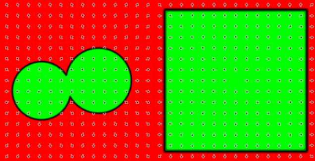
This diagram shows the standard distance visualisation’ for 2 fields used earlier in this blog. Overlaid are arrows that show the gradient. Inside the field, where the distance is negative, the gradient points directly towards the edge. Outside it, the gradient points directly away from the edge. These directions can be expressed as a 2D vector, which is referred to as the gradient vector. In a signed distance field, that vector is always of unit length (more on this later).

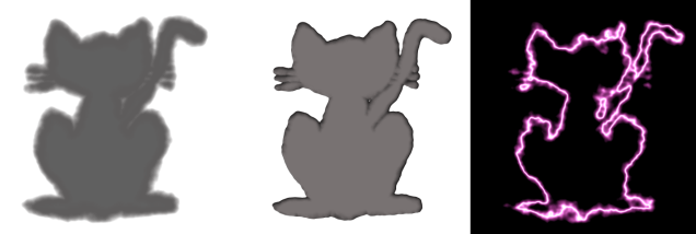
The gradients for our cat can be visualised for in a couple of ways:

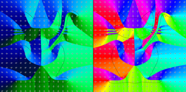
On the left, gradient.x (-1 to 1) is shown in the green channel and gradient.y (-1 to 1) is shown in the blue channel. My favoured visualisation on the right converts the gradient to an angle between 0 and 360 degrees, then uses the result to calculate a hue.

This next bit is a little mathematical, so if you don’t care about it, just know that:

• The gradient of a point represents the direction towards (if outside the geometry) or away from (if inside the geometry) the closest edge
• The gradient of a signed distance field is always a unit vector
• We’re updating SignedDistanceFieldGenerator.End() to calculate and store the gradient vector in the green and blue channels of the field texture
• To improve the field quality, I will also briefly introduce (but not go over in full) an improvement to our existing sweeping algorithm called an Eikonal Sweep

If you like, skip to the next section about bevels, or read on for some theory and codez!

Some theory

Calculation of the gradient requires a new concept – the partial derivatives of the field in x and y. This complex sounding term actually just means the rate of change in the x direction, and the rate of change in the y direction. To begin, assume the following definitions:

• The distance stored in the pixel at coordinate [i,j] is referred to as U_i,j
• The left neighbour at [i-1,j] is referred to as U_i-1,j
• The right neighbour at [i+1,j] is referred to as U_i+1,j
• The bottom neighbour at [i,j-1] is referred to as U_i,j-1
• The top neighbour at [i,j+1] is referred to as U_i,j+1

With these in mind, now consider the rate of change in X. To calculate it, we need to choose which neighbour (left or right) is closer to the edge (i.e. which is smaller).

• The smallest horizontal neighbour will be referred to as U_H
• If the left neighbour (U_i-1,j) is smallest, U_H = U_i-1,j and delta X (or dX) is -1
• If the right neighbour (U_i+1,j) is smallest, U_H = U_i+1,j and delta X (or dX) is +1
• The change in distance, U_H-U_i,j is called delta U, or dU
• Finally, the partial derivative in X is dU divided by dX, written dU/dX

In pseudo code:

GetPartialDerivativeInX(X,Y)
    //read Uij, Ui-1,j and Ui+1,j
    distance = GetDistance(X,Y) //Uij
    leftNeighbour = GetDistance(X-1,Y) //Ui-1,j
    rightNeighbour = GetDistance(X+1,Y) //Ui+1,j
    
    //choose either left or right neighbour to calculate
    //deltaU and deltaX
    if leftNeighbour < rightNeighbour:
        dU = leftNeighbour - distance 
        dX = -1
    else
        dU = rightNeighbour - distance 
        dX = 1
    end 

    //return the result 
    return dU/dX
end

We can do exactly the same for the partial derivative in Y (dU/dY), by calculating the smallest vertical neighbour (U_V) and executing the same logic. Pseudo code for the partial derivative in Y is thus:

GetPartialDerivativeInY(X,Y)
    //read Uij, Ui,j-1 and Ui,j+1
    distance = GetDistance(X,Y) //Uij
    bottomNeighbour = GetDistance(X,Y-1) //Ui,j-1
    topNeighbour = GetDistance(X,Y+1) //Ui,j+1
    
    //choose either top or bottom neighbour to calculate
    //deltaU and deltaX
    if bottomNeighbour < topNeighbour:
        dU = bottomNeighbour - distance 
        dY = -1
    else
        dU = topNeighbour - distance 
        dY = 1
    end 

    //return the result 
    return dU/dY
end

The gradient (or derivative) is simply a vector that contains [dU/dX, dU/dY]. For an SDF this should naturally be of unit length and not need to be normalized. Thus, in psuedo code:

GetGradient(X,Y)
    return [GetPartialDerivativeInX(X,Y),GetPartialDerivativeInY(X,Y)]
end

Hopefully that wasn’t too tricky, but if it was, don’t worry – as with most things in game dev, using it is more important than instantly getting the theory.

Calculating the gradient in code

Next, we’ll update SignedDistanceFieldGenerator.End() to iterate over every pixel, calculate the gradient vectors, and store them using the green and blue channels of the field texture:

for (int y = 0; y < m_y_dims; y++) {     for (int x = 0; x = 0 ? 1.0f : -1.0f;         float maxval = float.MaxValue * sign;         //read neighbour distances, ignoring border pixels         float x0 = x > 0 ? GetPixel(x - 1, y).distance : maxval;
        float x1 = x  0 ? GetPixel(x, y - 1).distance : maxval;
        float y1 = y < (m_y_dims - 1) ? GetPixel(x, y + 1).distance : maxval;

        //use the smallest neighbour in each direction to calculate the partial deriviates
        float xgrad = sign*x0 < sign*x1 ? -(x0-d) : (x1-d);
        float ygrad = sign*y0 < sign*y1 ? -(y0-d) : (y1-d);

        //combine partial derivatives to get gradient
        Vector2 grad = new Vector2(xgrad, ygrad);

        //store distance in red channel, and gradient in green/blue channels
        Color col = new Color();
        col.r = d;
        col.g = grad.x;
        col.b = grad.y;
        col.a = d < 999999f ? 1 : 0;
        cols[y * m_x_dims + x] = col;
    }
}

The code above is mostly a condensed version of the pseudo code to calculate the partial derivatives in X and Y, then combine them into a Vector2 gradient for every pixel. The only additions are:

• We use the sign of the source pixel to ensure all comparisons work correctly for inner (-ve) pixels
• Borders are handled by just assigning a ‘really big number’ to pixel coordinates that are out of bounds
• As a shortcut for dividing dU by 1 or -1, we just do/don’t negate it respectively
• And of course, the result, along with the distance is written into a colour for storage in a texture

Reminder: Find the full function in SignedDistanceFieldGenerator.cs

Improved field sweeping

One subtle issue I’ve mostly avoided up until now is that our current technique for sweeping isn’t perfect. When first introducing the 8PSSEDT sweeping algorithm, I showed this diagram:

It demonstrates how the approximation of A’s distance based on its neighbour (B) isn’t perfect. Mathematically, we end up with a gradient that points in slightly the wrong direction, and a distance that is slightly larger than it needs to be.

The sweep is most accurate close to the edge of the geometry (where the data is perfect) and gets worse as it moves outwards. Thus most of our distance effects haven’t really suffered. However if we render the contours of the field in blue, the issue is visible:

Note how further from the edge of the geometry, the sweep introduces straight contours, rather than nice curvy ones that match the geometry.

Some gradient effects are very sensitive to field accuracy, so I’ve added a new sweeping algorithm for this post called an Eikonal Sweep. This yields accurate distances and gradients, resulting in much nicer contours:

Eikonal sweeping is a much more mathematical approach and requires a whole post in itself, so I won’t cover it here. For now, know that a new EikonalSweep() function has been added to SignedDistanceFieldGenerator, to replace the existing Sweep() function.

Bevels

The bevel effect gives an image a fake 3D effect, by adding borders that are shaded in such a way as to look like they are edges:

This rather fancy looking border can do wonders for UI, and if used cleverly can even fake interaction with the lighting from the game world. The basic idea, as shown in the code below, is to use the gradient of the field with a pretend ‘light direction’ to shade the border:

//sample distance as normal
float d = sdf.r + _Offset;

//choose a light direction (just [0.5,0.5]), then dot product
//with the gradient to get a brightness
float2 lightdir = normalize(float2(0.5,0.5));
float diffuse = saturate(dot(sdf.gb,-lightdir));

//by default diffuse is linear (flat edge). combine with border distance
//to fake curvy one if desired
float curvature = pow(saturate(d/_BorderWidth),_BevelCurvature);
diffuse = lerp(1,diffuse,curvature);

//calculate the border colour (diffuse contributes 75% of 'light')
float4 border_col = _Fill * (diffuse*0.75+0.25);
border_col.a = 1;

//choose output
if(d < 0)
{
    //inside the goemetry, just use fill
    res = _Fill;
}
else if(d < _BorderWidth)
{
    //inside border, use border_col with tiny lerp across 1 pixel 
    //to avoid aliasing
    res = lerp(_Fill,border_col,saturate(d));
}
else
{
    //outside border, use fill col, with tiny lerp across 1 pixel 
    //to avoid aliasing 
    res = lerp(border_col,_Background,saturate(d-_BorderWidth));
}

Starting with the first bit:

//sample distance as normal
float d = sdf.r + _Offset;

//choose a light direction (just [0.5,0.5]), then dot product
//with the gradient to get a brightness
float2 lightdir = normalize(float2(0.5,0.5));
float diffuse = saturate(dot(sdf.gb,-lightdir));

This little section is the key to the whole effect. We pick a pretend ‘light direction’ (which could have been passed in as a shader parameter if desired), and dot product it with the gradient of the field. If the gradient directly opposes the light direction, it is assumed to be facing towards the light. If the gradient is perfectly aligned to the light direction, it is facing away from the light. On completion, diffuse contains a value between 0 and 1 indicating how lit the border is at this point.

Skipping over the curvature section for the moment, we then calculate the actual colour of the border.

//calculate the border colour (diffuse contributes 75% of 'light')
float4 border_col = _Fill * (diffuse*0.75+0.25);
border_col.a = 1;

This simple code selects the border colour by applying our lighting to the fill colour. The lighting is effectively taking 25% ambient light, and 75% of the diffuse light.

Finally, probably familiar by now, we select whether to use background, border or fill colour:

//choose output
if(d < 0)
{
    //inside the goemetry, just use fill
    res = _Fill;
}
else if(d < _BorderWidth)
{
    //inside border, use border_col with tiny lerp across 1 pixel 
    //to avoid aliasing
    res = lerp(_Fill,border_col,saturate(d));
}
else
{
    //outside border, use fill col, with tiny lerp across 1 pixel 
    //to avoid aliasing 
    res = lerp(border_col,_Background,saturate(d-_BorderWidth));
}

This is simply choosing _Fill if inside the shape, border_col if within the border, or _Background otherwise. The lerps serve no purpose for the effect other than to avoid aliasing by transitioning cleanly between colours over 1 pixel.

If we were to just use this code, ignoring the curvature section, the result is already visibily ‘3D’:

The extra ‘curvature’ section just tweaks the diffuse lighting value based on distance from the edge of the geometry:

//by default diffuse is linear (flat edge). combine with border distance
//to fake curvy one if desired
float curvature = pow(saturate(d/_BorderWidth),_BevelCurvature);
diffuse = lerp(1,diffuse,curvature);

If _BevelCurvature is 0, curvature will always equal 1. As a result, the lerp will never change the value of diffuse. However, as _BevelCurvature increases, the distance, d, the pixel is from the edge will have an increasingly large effect. This causes diffuse to be increasingly biased towards a value of 1 close to the edge of the geometry. Visually, this produces a curvy look, rather than an angular look:

The one remaining problem you may have spotted is the unpleasant discontinuities in the shading:

These unfortunate artefacts are a result of the fact that our source image simply wasn’t of a high enough quality to get good gradients out. Despite our efforts, the conversion from image to field isn’t perfect and the issue shows up when using gradient based effects. A high curvature tends to hide the issue a little, but the artefact is always there.

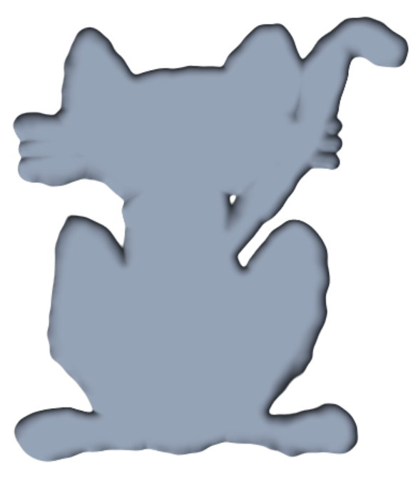
The most obvious solution is to use a very high resolution source image and then downsample. However, if not practical, one option is to blur the field slightly. This will make it less accurate in terms of distances, but soften out ‘crinkles’ in the field. I have added to SignedDistanceFieldGenerator a very simple Soften() function that applies a dumb blur to every pixel to demo the effect:

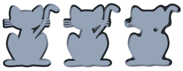
As you can see, the subtle blur in the middle has little effect on the shape of the geometry, but does get rid of the artefacts. On the right the blur is turned right up which results in a blobby field (a fun effect in itself!). Note: please ignore the the fact that the lighting is inverted on the left image – shader bug when taking screen shots!

Whether softening is the right solution for you will depend on your scenario. Ideally for high quality data you start from high quality input assets, but if that’s not practical, sacrificing field accuracy for smoothness may be a good way to go.

Note: if you do decide to rely on softening, I recommend looking up better algorithms than the supplied Soften function, as I knocked it together in 10 minutes and it isn’t very smart!

Finding The Edge

The addition of gradient info to the field yields another handy property – a given point, with both the distance and direction to/from the closest edge, it is easy to find out the actual location of the closest edge. Whilst this isn’t so much an effect, it’s a useful feature and can generate some fun visualisations.

In this diagram we start off with sampling a distance field at a location, p = [1.5,1.5]. At this location, the distance field tells us:

• the closest edge is at a distance, d = 3.53 away
• the gradient, which points directly away from the closest edge, is g =[-0.71,-0.71

Armed with this information, it is easy to see that to get the location of the closest edge point we multiply the gradient by distance and subtract from the input point. Mathematically:

edge point, ep = p – d * g

Or in psuedo code:

GetClosestEdgePoint(Vector2 SrcPoint)
    //read distance,d and gradient,g from field
    Float Distance,Gradient;
    SampleField(SrcPoint, out Distance, out Gradient)

    //calculate and return point
    return SrcPoint - Distance * Gradient
End

We can visualise the results of edge finding by:

• Sampling the SDF at a given UV as normal
• Working out the corresponding edge UV
• Sampling the SDF at the edge UV

If our logic is valid the edge sample should return a distance very close to 0 (as it is the edge!). To begin, we’ll create a function to find and sample the edge:

void sampleedge(float4 sdf, float2 uv, out float4 edgesdf, out float2 edgeuv)
{
    edgeuv = uv - sdf.gb*sdf.r*_MainTex_TexelSize.xy;
    edgesdf = samplesdf(edgeuv);
}

Next, we’ll add a new edge finder visualization to the shader:

else if(_Mode == 12) //EdgeFind
{
    //use sampleedge to get the edge field values and uv
    float2 edgeuv;
    float4 edgesdf;
    sampleedge(sdf,uv,edgesdf,edgeuv);

    //visualize error threshold of 1 pixel in r, and highlight geometry edge with b
    float edged = edgesdf.x;
    res.r = abs(edged) > 1 ? 1 : 0;
    res.g = 0;
    res.b = 1-saturate(abs(sdf.r));
}

This simple shader samples the edge distance field, and outputs a red pixel if the error is greater than 1. As an extra tweak, it highlights the actual edge blue so we can still see the geometry:

The result, as you can see, is OK but far from perfect. Black pixels represent areas that successfully found the edge. However we can see distinct lines, worst on the cat, where the test failed. Comparing the edge finder to the gradient view it is possible to see where these errors occurred:

Any SDF contains discontinuities – areas where 2 neighbouring pixels have different closest edges. On the right hand image where the gradient is visualised, these discontinuities show up as sharp changes in colour. In the left image these correspond precisely to areas where edge finding failed.

The simplest way to solve this is to simply keep stepping toward the edge, getting a little bit closer each time:

bool GetClosestEdgePoint(Vector2 Point, int MaxSteps, out Result)
    For(i = 1 to MaxSteps)
        Float Distance,Gradient;
        SampleField(Point, out Distance, out Gradient)
        if(abs(Distance) < 0.5)
            break
        Point -= Distance * Gradient
    End
    Result = Point
    return abs(Distance) < 0.5
End

This pseudo code will iterate until a point has been found within 0.5 pixels or reaches a predefined maximum number of steps.

To implement it in the shader, we’ll introduce a new function called steptowardsedge, that takes as an input a sample and UV, then updates them both with a sample and UV closer to the edge:

void steptowardsedge(inout float4 edgesdf, inout float2 edgeuv)
{
    edgeuv -= edgesdf.gb*edgesdf.r*_MainTex_TexelSize.xy;
    edgesdf = samplesdf(edgeuv);
}

The sampleedge function is then updated to keep sampling until the edge is reached:

bool sampleedge(float4 sdf, float2 uv, out float4 edgesdf, out float2 edgeuv, out int steps)
{
    edgesdf = sdf;
    edgeuv = uv;
    steps = 0;

    [unroll(8)]
    for(int i = 0; i < _EdgeFindSteps; i++)
    {
        if(abs(edgesdf.r) < 0.5)
            break;
        steptowardsedge(edgesdf,edgeuv);
        steps++;
    }

    return abs(edgesdf.r) < 0.5;
}

This new version also returns true/false to indicate whether the edge was found, and outputs the number of steps taken. Using this new data, we can update the edge find visualisation to render a hue that shows how many steps were taken, or simply shows black if the edge was never found:

else if(_Mode == 12) //EdgeFind
{
    //use sampleedge to get the edge field values and uv
    float2 edgeuv;
    float4 edgesdf;
    int edgesteps;
    bool success = sampleedge(sdf,uv,edgesdf,edgeuv,edgesteps);

    //visualize number of steps to reach edge (or black if didn't get there')
    res.rgb = success ? HUEtoRGB(0.75f*edgesteps/8.0f) : 0;
}

Running this visualisation on the cat field gives us this image:

Here we see:

• Red pixels took 0 steps – i.e. they are already on the edge
• Orange pixels (the majority) took 1 step
• Yellow pixels took 2 steps
• Green pixels took 3 steps
• No black pixels are visible, as the edge never failed to be found

This technique can also be handy if you’re dealing with a less accurate field, having softened it to reduce artefacts as mentioned in the bevels section:

Here you can see many more pixels had to take 2 steps (yellow) due to the less accurate field, however they still all got there eventually.

Noise

Noise based effects aren’t specific to SDFs, but they certainly work well together. In case you’re not familiar with the concept of noise, it typically refers to a way of generating a grid of values that whilst random, are still continuous (think clouds instead of static):

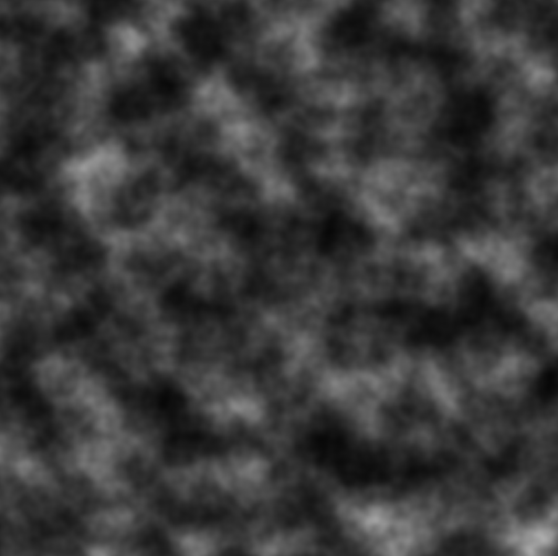
Above is a noise texture, generated by layering Perlin Noise at different frequencies, named after the father of this technique – Ken Perlin. I don’t want to go into too much depth on how noise works for this blog though – the key is, we’ve got a texture like the one above! In fact, we have a 4 channel texture, with a different ‘cloud pattern’ stored in each channel.

For reference, the function that generates it works by sampling Unity’s built in Perlin noise in multiple octaves:

Color[] GenerateNoiseGrid(int w, int h, int octaves, float frequency, float lacunarity, float persistance)
{
    //calculate scalars for x/y dims
    float xscl = 1f / (w - 1);
    float yscl = 1f / (h - 1);

    //allocate colour buffer then iterate over x and y
    Color[] cols = new Color[w * h];
    for (int x = 0; x < w; x++)
    {
        for (int y = 0; y < h; y++)
        {
            //classic multi-octave perlin noise sampler
            //ends up with 4 octave noise samples
            Vector4 tot = Vector4.zero;
            float scl = 1;
            float sum = 0;
            float f = frequency;
            for (int i = 0; i < octaves; i++)
            {
                for (int c = 0; c < 4; c++)
                    tot[c] += Mathf.PerlinNoise(c * 64 + f * x * xscl, f * y * yscl) * scl;
                sum += scl;
                f *= lacunarity;
                scl *= persistance;
            }
            tot /= sum;

            //store noise value in colour
            cols[y * w + x] = new Color(tot.x, tot.y, tot.z, tot.w);
        }
    }
    return cols;
}

This function is used to generate the pixel colours for a texture, which is then stored in the SDF class as m_noise_texture, and passed into the shader as _NoiseTex.

We then have a tiny function in the shader that samples the 4 channel texture, and combines each channel into a single animated value.

//samples the animated noise texture
float samplenoise(float2 uv)
{
    float t = frac(_NoiseAnimTime)*2.0f*3.1415927f;
    float k = 0.5f*3.1415927f;
    float4 sc = float4(0,k,2*k,3*k)+t;
    float4 sn = (sin(sc)+1)*0.4;       
    return dot(sn,tex2D(_NoiseTex,uv));
}

Although it looks a little funky, all this function is really doing is taking a parameter called _NoiseAnimTime and using it to generate a vector, sn that contains 4 different values between 0 and 1. This is then combined with the sampled _NoiseTex to get an output noise value between 0 and 1 that animates over time:

A cleverer but more expensive approach might have been to fully generate noise within the shader. This is entirely achievable on modern GPUs, but impractical on lower end mobile devices.

Now we’re going to use the output of this samplenoise function within the samplesdf function to modify the sampled distance. Our sample function now looks like this:

//helper to perform the sdf sample 
float4 samplesdf(float2 uv)
{
      //sample distance field
    float4 sdf = tex2D(_MainTex, uv);

    //if we want to do the 'circle morph' effect, lerp from the sampled 
    //value to a circle value here
    if(_CircleMorphAmount > 0)
    {
        float4 circlesdf = centeredcirclesdf(uv,_CircleMorphRadius);
        sdf = lerp(sdf, circlesdf, _CircleMorphAmount);
    }

    //re-normalize gradient in gb components as bilinear filtering
    //and the morph can mess it up 
    sdf.gb = normalize(sdf.gb);
                
    //if edge based noise is on, adjust distance by sampling noise texture
    if(_EnableEdgeNoise)
    {
        sdf.r += lerp(_EdgeNoiseA,_EdgeNoiseB,samplenoise(uv));
    }
                
    return sdf;
}
    

Assuming _EnableEdgeNoise is true, the updated function now:

• Reads a noise value from 0 to 1
• Uses it to lerp between 2 input parameters: _EdgeNoiseA and _EdgeNoiseB
• Adds the result to the sampled distance

As all our effects work by calling samplesdf, they will now all support reading the ‘noisy’ distances. Playing with different effects and noise values, the results can be very varied and quite pleasing:

And of course, because it’s animated…

A note on broken fields

It’s worth mentioning at this point that both the earlier morph effect, and our updated noise effect break the field a little. By this I mean that after fiddling with the sampled values they are no longer guaranteed to represent the distance to the closest edge. This is surprisingly well hidden with most of the effects so far, as they only really care about values very close to the edge of the geometry where the errors are smallest. However, we can spot the result in the bevel effect:

One result of the broken field is that our calculated gradient values no longer match those of the field with noisy edges applied. As a result, the wibbly edge is still shaded as though it were flat.

There are many approaches to solving this issue depending on your use case. At the extreme end, you might perform your morphing or noise on the CPU, then do a full re-sweep of the field every frame. On the other hand, if the problem isn’t particularly visible, you might do nothing at all!

For this particular situation, we’re going to ignore the distance errors, but attempt to fix the gradient on the fly so the bevel works nicely. To do so, we’ll add a new function to the shader designed to only sample the distance, but ignore gradient:

//cut down version of samplesdf that ignores gradient
float samplesdfnograd(float2 uv)
{
      //sample distance field
    float4 sdf = tex2D(_MainTex, uv);

    //if we want to do the 'circle morph' effect, lerp from the sampled 
    //value to a circle value here
    if(_CircleMorphAmount > 0)
    {
        float4 circlesdf = centeredcirclesdf(uv,_CircleMorphRadius);
        sdf = lerp(sdf, circlesdf, _CircleMorphAmount);
    }
                
    //if edge based noise is on, adjust distance by sampling noise texture
    if(_EnableEdgeNoise)
    {
        sdf.r += lerp(_EdgeNoiseA,_EdgeNoiseB,samplenoise(uv));
    }

    return sdf;      
}

That should look pretty familiar! Now, we’ll add the following lines to the main sdf sampling function:

    //if requested, overwrite sampled gradient with one calculated live in
    //shader that takes into account morphing and noise
    if(_FixGradient)
    {
        float d = sdf.r;
        float sign = d > 0 ? 1 : -1;
        float x0 = samplesdfnograd(uv+_MainTex_TexelSize.xy*float2(-1,0));
        float x1 = samplesdfnograd(uv+_MainTex_TexelSize.xy*float2(1,0));
        float y0 = samplesdfnograd(uv+_MainTex_TexelSize.xy*float2(0,-1));
        float y1 = samplesdfnograd(uv+_MainTex_TexelSize.xy*float2(0,1));
               
        float xgrad = sign*x0 < sign*x1 ? -(x0-d) : (x1-d);
        float ygrad = sign*y0 < sign*y1 ? -(y0-d) : (y1-d);
                
        sdf.gb = float2(xgrad,ygrad);
    }

This rather expensive function performs the same calculations within the shader that our earlier CPU code used to calculate the gradient by sampling neighbours. However, by being run in the shader and accounting for morphing / noise, it provides much more accurate gradients:

Note the shading on the wobbly edges now contains matching shadows.

Summary

That concludes what I think is probably the main section my intro to SDFs. Across the 7 posts you should have learnt the core principles of signed distance fields and seen how they can be used in 2D to generate some useful effects. Some future things to look at that I may cover, or you may wish to investigate are:

• 3D fields. These work exactly like 2D fields in every way! Visualising them can be tricky though. A good place to start is to search for the marching cubes or marching tetrahedrons algorithms online.
• Physics. Signed distance fields are ideally suited to collision detection and ray casting, as they make it very easy to find out the distance to an edge from any given point. If you’re looking at making a game with very bumpy or modifiable terrain, SDFs are ideal.
• CSG (constructive solid geometry) is the technique of combining shapes in different ways (primarily ‘add’ and ‘subtract’) to get more complex geometry.
• Lighting. Both in 3D and 2D, using distance fields to represent lighting volumes can be a very effective way of generating complex dynamic lighting in a scene.
• Sparse fields. In 3D especially fields can get very memory hungry. However many have used a technique in which fields are stored in a tree, with high resolution data only maintained close to the surface of geometry.
• Compression. Throughout this blog we’ve stored data in fairly expensive floating point textures. A simple modification is to store field distances in classic 1 byte per channel textures. This is achieved by storing distances as values between 0 and 1, then rescaling them to cover large signed ranges.

Maybe if I get some requests I’ll cover some of those at some point. Until then, enjoy the code here:

https://github.com/chriscummings100/signeddistancefields

Enjoy!